Appendix to Subpart H—Calibrating the GSIB Surcharge*
Abstract
This white paper discusses how to calibrate a capital
surcharge that tracks the systemic footprint of a global systemically
important bank holding company (GSIB). There is no widely accepted
calibration methodology for determining such a surcharge. The white
paper focuses on the “expected impact” framework, which is based on
each GSIB’s expected impact on the financial system, understood as
the harm it would cause to the financial system were it to fail multiplied
by the probability that it will fail. Because a GSIB’s failure would
cause more harm than the failure of a non-GSIB, a GSIB should hold
enough capital to lower its probability of failure so that its expected
impact is approximately equal to that of a non-GSIB.
Applying the expected impact framework requires
several elements. First, it requires a method for measuring the relative
harm that a given banking firm’s failure would cause to the financial
system—that is, its systemic footprint. This white paper uses the
two methods as set forth in the GSIB surcharge rule to quantify a
firm’s systemic impact. Those methods look to attributes of a firm
that are drivers of its systemic importance, such as size, interconnectedness,
and cross-border activity. Both methodologies use the most recent
data available, and firms’ scores will change over time as their systemic
footprints change. Second, the expected impact framework requires
a means of estimating the probability that a firm with a given level
of capital will fail. This white paper estimates that relationship
using historical data on the probability that a large U.S. banking
firm will experience losses of various sizes. Third, the expected
impact framework requires the choice of a “reference” bank holding
company: A large, non-GSIB banking firm whose failure would not pose
an outsized risk to the financial system. This white paper discusses
several plausible choices of reference BHC.
With these elements, it is possible to estimate a capital
surcharge that would reduce a GSIB’s expected impact to that of a
non-GSIB reference BHC. For each choice of reference BHC, the white
paper provides the ranges of reasonable surcharges for each U.S. GSIB.
Introduction
The Dodd-Frank Wall Street Reform and Consumer Protection Act1 mandates
that the Board of Governors of the Federal Reserve System adopt, among
other prudential measures, enhanced capital standards to mitigate
the risk posed to financial stability by systemically important financial
institutions (SIFIs). The Board has already implemented a number of
measures designed to strengthen firms’ capital positions in a manner
consistent with the Dodd-Frank Act’s requirement that such measures
increase in stringency based on the systemic importance of the firm.
As part of this process, the Board has proposed a set
of capital surcharges to be applied to the eight U.S. bank holding
companies (BHCs) of the greatest systemic importance, which have been
denominated global systemically important bank holding companies (GSIBs).
Setting such an enhanced capital standard entails (1) measuring the
risk that a given GSIB’s failure poses to financial stability (that
is, the GSIB’s systemic footprint) and (2) estimating how much
additional capital is needed to mitigate the systemic risk posed by
a firm with a given systemic footprint.
This white paper explains the calibration of the capital
surcharges, based on the measures of each GSIB’s systemic footprint
derived from the two methods described in the GSIB surcharge final
rule and discussed in detail in the preamble to the rule. Because
there is no single widely accepted framework for calibrating a GSIB
surcharge, the Board considered several potential approaches. This
paper focuses on the “expected impact” framework, which is the most
appropriate approach for helping to scale the level of a capital surcharge.
This paper explains the expected impact framework in detail. It provides
surcharge calibrations resulting from that framework under a range
of plausible assumptions, incorporating the uncertainty that is inherent
in the study of rare events such as systemic banking failures. This
paper also discusses, at a high level, two alternative calibration
frameworks, and it explains why neither seemed as useful as a framework
for the calibration of the GSIB surcharge.
Background
The failures and
near-failures of SIFIs were key drivers of the 2007-08 financial crisis
and the resulting recession. They were also key drivers of the public-sector
response to the crisis, in which the United States government sought
to prevent SIFI failures through extraordinary measures such as the
Troubled Asset Relief Program. The experience of the crisis made clear
that the failure of a SIFI during a period of stress can do great
damage to financial stability, that SIFIs themselves lack sufficient
incentives to take precautions against their own failures, that reliance
on extraordinary government interventions going forward would invite
moral hazard and lead to competitive distortions, and that the pre-crisis
regulatory focus on microprudential risks to individual financial
firms needed to be broadened to include threats to the overall stability
of the financial system.
In keeping with these lessons, post-crisis regulatory
reform has placed great weight on “macroprudential” regulation, which
seeks to address threats to financial stability. Section 165 of the
Dodd-Frank Act pursues this goal by empowering the Board to establish
enhanced regulatory standards for “large, interconnected financial
institutions” that “are more stringent than the standards . . . applicable
to [financial institutions] that do not present similar risks to the
financial stability of the United States” and “increase in stringency”
in proportion to the systemic importance of the financial institution
in question.2 Section 165(b)(1)(A)(i) of the act points
to risk-based capital requirements as a required type of enhanced
regulatory standard for SIFIs.
Rationales for a GSIB Surcharge
The Dodd-Frank
Act’s mandate that the Board adopt enhanced capital standards to mitigate
the risk posed to financial stability by certain large financial institutions
provides the principal statutory impetus for enhanced capital requirements
for SIFIs. Because the failure of a SIFI could undermine financial
stability and thus cause far greater negative externalities than could
the failure of a financial institution that is not systemically important,
a probability of default that would be acceptable for a non-systemic
firm may be unacceptably high for a SIFI. Reducing the probability
that a SIFI will default reduces the risk to financial stability.
The most straightforward means of lowering a financial firm’s probability
of default is to require it to hold a higher level of capital relative
to its risk-weighted assets than non-SIFIs are required to hold, thereby
enabling it to absorb greater losses without becoming insolvent.
There are also two secondary rationales for enhanced capital
standards for SIFIs. First, higher capital requirements create incentives
for SIFIs to shrink their systemic footprint, which further reduces
the risks these firms pose to financial stability. Second, higher
capital requirements may offset any funding advantage that SIFIs have
on account of being perceived as “too big to fail,” which reduces
the distortion in market competition caused by the perception and
the potential that counterparties may inappropriately shift more risk
to SIFIs, thereby increasing the risk those firms pose to the financial
system. Increased capital makes GSIBs more resilient in times of economic
stress, and, by increasing the capital cushion available to the firm,
may afford the firm and supervisors more time to address weaknesses
at the firm that could reverberate through the financial system were
the firm to fail.
The
Expected Impact Framework
By definition, a
GSIB’s failure would cause greater harm to financial stability than
the failure of a banking organization that is not a GSIB.3 Thus, if
all banking organizations are subject to the same risk-based capital
requirements and have similar probabilities of default, GSIBs will
impose far greater systemic risks than non-GSIBs will. The expected
impact framework addresses this discrepancy by subjecting GSIBs to
capital surcharges that are large enough that the expected systemic
loss from the failure of a given GSIB better approximates the expected
systemic loss from the failure of a BHC that is large but is not a
GSIB. (We will call this BHC the “reference BHC.”)
The expected loss from a given firm’s failure
can be computed as the systemic losses that would occur if that firm
failed, discounted by the probability of its failure. Using the acronyms
LGD (systemic loss given default), PD (probability of default), and
EL (expected loss), this idea can be expressed as follows: EL =
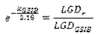
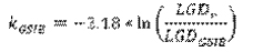
LGD * PD
The goal of a GSIB surcharge is to equalize the expected
loss from a GSIB’s failure to the expected loss from the failure of
a non-GSIB reference BHC: ELGSIB= ELr
By definition, a GSIB’s LGD is higher than that of a non-GSIB.
So to equalize EL between GSIBs and non-GSIBs, we must require each
GSIB to lower its PD, which we can do by requiring it to hold more
capital.
This implies that a GSIB must increase its capital level
to the extent necessary to reach a PD that is as many times lower
than the PD of the reference BHC as its LGD is higher than the LGD
of the reference BHC. (For example, suppose that a particular GSIB’s
failure would cause twice as much loss as the failure of the reference
BHC. In that case, to equalize EL between the two firms, we must require
the GSIB to hold enough additional capital that its PD is half that
of the reference BHC.) That determination requires the following components,
which we will consider in turn:
1. A method for creating “LGD scores” that
quantify the GSIBs’ LGDs
2. An LGD score for the reference BHC
3. A function relating a firm’s capital
ratio to its PD
Quantifying GSIB LGDs
The final rule employs two methods to measure GSIB
LGD:
Method 1 is based on the internationally accepted
GSIB surcharge framework, which produces a score derived from a firm’s
attributes in five categories: Size, interconnectedness, complexity,
cross-jurisdictional activity, and substitutability.
Method 2 replaces method 1’s substitutability category
with a measure of a firm’s reliance on short-term wholesale funding.
The preambles to the GSIB surcharge notice of proposed
rulemaking and final rule explain why these categories serve as proxies
for the systemic importance of a banking organization (and thus the
systemic harm that its failure would cause). They also explain how
the categories are weighted to produce scores under method 1 and method
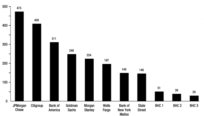
2. Table 1 conveys the Board’s estimates of the current scores for
the eight U.S. BHCs with the highest scores. These scores are estimated
from the most recent available data on firm-specific indicators of
systemic importance. The actual scores that will apply when the final
rule takes effect may be different and will depend on the future evolution
of the firm-specific indicator values.
Table 1—Top
eight scores under each method
Firm
Method 1 score
Method 2 score
JPMorgan Chase
473
857
Citigroup
409
714
Bank of America
311
559
Goldman Sachs
248
585
Morgan Stanley
224
545
Wells Fargo
197
352
Bank of New York
Mellon
149
213
State Street
146
275
This paper assumes that the relationships between the
scores produced by these methods and the firms’ systemic LGDs are
linear. In other words, it assumes that if firm A’s score is twice
as high as firm B’s score, then the systemic harms that would flow
from firm A’s failure would be twice as great as those that would
flow from firm B’s failure.
In fact, there is reason to believe that firm A’s failure
would do more than twice as much damage as firm B’s. (In other words,
there is reason to believe that the function relating the scores to
systemic LGD increases at an increasing rate and is therefore nonlinear.)
The reason is that at least some of the components of the two methods
appear to increase the systemic harms that would result from a default
at an increasing rate, while none appears to increase the resulting
systemic harm at a decreasing rate. For example, because the negative
priceimpact associated with the fire-sale liquidation of certain asset
portfolios increases with the size of the portfolio, systemic LGD
appears to grow at an increasing rate with the size, complexity, and
short-term wholesale funding metrics used in the methods. Thus, this
paper’s assumption of a linear relationship simplifies the analysis
while likely resulting in surcharges lower than those that would result
if the relationship between scores and systemic LGD were assumed to
be non-linear.
The Reference BHC’s Systemic LGD
Score
The reference BHC is a real or hypothetical
BHC whose LGD will be used in our calculations. The expected impact
framework requires that the reference BHC be a non-GSIB, but it leaves
room for discretion as to the reference BHC’s identity and LGD score.
Potential Approaches
The reference BHC score can be viewed as simply the LGD
score which, given the PD associated with the generally applicable
capital requirements, produces the highest EL that is consistent with
the purposes and mandate of the Dodd-Frank Act. The effect of setting
the reference BHC score to that LGD score would be to hold all GSIBs
to that EL level. The purpose of the Dodd-Frank Act is “to prevent
or mitigate risks to the financial stability of the United States
that could arise from the material financial distress or failure,
or ongoing activities, of large, interconnected financial institutions.”4 The following options appear to be conceptually
plausible ways of identifying the reference BHC for purposes of establishing
a capital requirement for GSIBs that lowers the expected loss from
the failure of a GSIB to the level associated with the failure of
a non-GSIB.
Option 1: A BHC with $50 billion in assets. Section
165(a)(1) of the Dodd-Frank Act calls for the Board to “establish
prudential standards for . . . bank holding companies with total consolidated
assets equal to or greater than $50,000,000,000 that (A) are more
stringent than the standards . . . applicable to . . . bank holding
companies that do not present similar risks to the financial stability
of the United States; and (B) increase in stringency.” Section 165
is the principal statutory basis for the GSIB surcharge, and its $50
billion figure provides a line below which it may be argued that Congress
did not believe that BHCs present sufficient “risks to the financial
stability of the United States” to warrant mandatory enhanced prudential
standards. It would therefore be reasonable to require GSIBs to hold
enough capital to reduce their expected systemic loss to an amount
equal to that of a $50 billion BHC that complies with the generally
applicable capital rules. Although $50 billion BHCs could have a range
of LGD scores based upon their other attributes, reasonable score
estimates for a BHC of that size are 3 under method 1 and 37 under
method 2.5
Option 2: A BHC with $250 billion in assets. The
Board’s implementation of the advanced approaches capital framework
imposes enhanced requirements on banking organizations with at least
$250 billion in consolidated assets. This level distinguishes the
largest and most internationally active U.S. banking organizations,
which are subject to other enhanced capital standards, including the
countercyclical capital buffer and the supplementary leverage ratio.6 The $250 billion threshold therefore provides another viable line
for distinguishing between the large, complex, internationally active
banking organizations that pose a substantial threat to financial
stability and those that do not pose such a substantial threat. Although
$250 billion BHCs could have a range of LGD scores based upon their
other attributes, reasonable score estimates for a BHC of that size
are 23 under method 1 and 60 under method 2.7
Option 3: The U.S. non-GSIB with the highest LGD score. Another plausible reference BHC is the actual U.S. non-GSIB BHC
that comes closest to being a GSIB—in other words, the U.S. non-GSIB
with the highest LGD score. Under method 1, the highest score for
a U.S. non-GSIB is 51 (the second-highest is 39). Under method 2,
the highest score for a U.S. non-GSIB is estimated to be 85 (the second-
and third-highest scores are both estimated to be 75).8
Option 4: A hypothetical BHC at the cutoff line between
GSIBs and non-GSIBs. Given that BHCs are divided into GSIBs and
non-GSIBs based on their systemic footprint and that LGD scores provide
our metric for quantifying firms’ systemic footprints, there must
be some LGD score under each method that marks the “cut-off line”
between GSIBs and non-GSIBs. The reference BHC’s score should be no
higher than this cut-off line, since the goal of the expected impact
framework is to lower each GSIB’s EL so that it equals the EL of a
non-GSIB. Under this option, the reference BHC’s score should also
be no lower than the cut-off line, since if it were lower,
then a non-GSIB firm could exist that had a higher LGD and therefore
(because it would not be subject to a GSIB surcharge) a higher
EL than GSIBs are permitted to have. Under this reasoning, the reference
BHC should have an LGD score that is exactly on the cut-off line between
GSIBs and non-GSIBs. That is, it should be just on the cusp of being
a GSIB.
What LGD score marks the cut-off line between GSIB and
non-GSIB? With respect to method 1, figure 1 shows that there is a
large drop-off between the eighth-highest score (146) and the ninth-highest
score (51). Drawing the cut-off line within this target range is reasonable
because firms with scores at or below 51 are much closer in size and
complexity to financial firms that have been resolved in an orderly
fashion than they are to the largest financial firms, which have scores
between three and nine times as high and are significantly larger
and more complex. We will choose a cut-off line at 130, which is at
the high end of the target range. This choice is appropriate because
it aligns with international standards and facilitates comparability
among jurisdictions. It also establishes minimum capital surcharges
that are consistent internationally.
Figure 1—Estimated
method 1 scores
Figure 1. Estimated method
1 scores
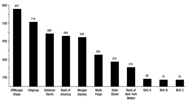
A similar approach can be used under method 2. Figure
2 depicts the estimated method 2 scores of the eleven U.S. BHCs with
the highest estimated scores. A large drop-off in the distribution
of scores with a significant difference in character of firms occurs
between firms with scores above 200 and firms with scores below 100.
The range between Bank of New York Mellon and the next-highest-scoring
firm is the most rational place to draw the line between GSIBs and
non-GSIBs: Bank of New York Mellon’s score is roughly 251 percent
of the score of the next highest-scoring firm, which is labeled BHC
A. (There is also a large gap between Morgan Stanley’s score and Wells
Fargo’s, but the former is only about 154 percent of the latter.)
This approach also generates the same list of eight U.S. GSIBs as
is produced by method 1. In selecting a specific line within this
range, we considered the statutory mandate to protect U.S. financial
stability, which argues for a method of calculating surcharges that
addresses the importance of mitigating the failure of U.S. GSIBs,
which are among the most systemic in the world. This would suggest
a cut-off line at the lower end of the target range. The lower threshold
is appropriate in light of the fact that method 2 uses a measure of
short-term wholesale funding in place of substitutability. Specifically,
short-term wholesale funding is believed to have particularly strong contagion
effects that could more easily lead to major systemic events, both
through the freezing of credit markets and through asset fire sales.
These systemic impacts support the choice of a threshold at the lower
end of the range for method 2.
Figure 2—Estimated
method 2 scores
Figure 2. Estimated method
2 scores
Although the failure of a firm with the systemic footprint
of BHC A poses a smaller risk to financial stability than does the
failure of one of the eight GSIBs, it is nonetheless possible that
the failure of a very large banking organization like BHC A, BHC B,
or BHC C could have a negative effect on financial stability, particularly
during a period of industry-wide stress such as occurred during the
2007-08 financial crisis. This provides additional support for our
decision to draw the line between GSIBs and non-GSIBs at 100 points,
at the lower end of the range between Bank of New York Mellon and
BHC A.
Note that we have set our method 2 reference BHC score
near the bottom of the target range and our method 1 reference BHC
score near the top of the target range. Due to the choice of reference
BHC in method 2, method 2 is likely to result in higher surcharges
than method 1. Calculating surcharges under method 1 in part recognizes
the international standards applied globally to GSIBs. Using a globally
consistent approach for establishing a baseline surcharge has benefits
for the stability of the entire financial system, which is globally
interconnected. At the same time, using an approach that results in
higher surcharges for most GSIBs is consistent with the statutory
mandate to protect financial stability in the United States and with
the risks presented by short-term wholesale funding.
Capital and Probability of Default
To implement
the expected impact approach, we also need a function that relates
capital ratio increases to reductions in probability of default. First,
we use historical data drawn from FR Y-9C regulatory reports from
the second quarter of 1987 through the fourth quarter of 2014 to plot
the probability distribution of returns on risk-weighted assets (RORWA)
for the 50 largest BHCs (determined as of each quarter), on a four-quarter
rolling basis.9 RORWA is defined as after-tax net income divided by risk-weighted
assets. Return on risk-weighted assets provides a better measure of
risk than return on total assets would, because the risk weightings
have been calibrated to ensure that two portfolios with the same risk-weighted
assets value contain roughly the same amount of risk, whereas two
portfolios with total assets of the same value can contain very different
amounts of risk depending on the asset classes in question.
We select this date range and set
of firms to provide a large sample size while focusing on data from
the relatively recent past and from very large firms, which are more
germane to our purposes. Data from the past three decades may be an
imperfect predictor of future trends, as there are factors that suggest
that default probabilities in the future may be either lower or higher
than would be predicted on the basis of the historical data.
On the one hand, these data do not
reflect many of the regulatory reforms implemented in the wake of
the 2007-08 financial crisis that are likely to reduce the probability
of very large losses and therefore the probability of default associated
with a given capital level. For example, the Basel 2.5 and Basel III
capital reforms are intended to increase the risk-sensitivity of the
risk weightings used to measure risk-weighted assets, which suggests
that the risk of losses associated with each dollar of risk-weighted
assets under Basel III will be lower than the historical, pre-Basel
III trend. Similarly, post-crisis liquidity initiatives (the liquidity
coverage ratio and the net stable funding ratio) should reduce the
default probabilities of large banking firms and the associated risk
of fire sales. Together, these reforms may lessen a GSIB’s probability
of default and potentially imply a lower GSIB surcharge.
On the other hand, however, extraordinary
government interventions during the time period of the dataset (particularly
in response to the 2007-08 financial crisis) undoubtedly prevented
or reduced large losses that many of the largest BHCs would otherwise
have suffered. Because one core purpose of post-crisis reform is to
avoid the need for such extraordinary interventions in the future,
the GSIB surcharge should be calibrated using data that include the
severe losses that would have materialized in the absence of such
intervention; because the interventions in fact occurred, using historical
RORWA data may lead us to underestimate the probability of default
associated with a given capital level. In short, there are reasons
to believe that the historical data underestimate the future trend,
and there are reasons to believe that those data overestimate the
future trend. Although the extent of the over- and underestimations
cannot be rigorously quantified, a reasonable assumption is that they
roughly cancel each other out.10
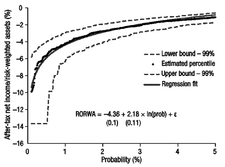
Figure 3 displays the estimated quantiles of ROWRA from
0.1 to 5.0. The sample quantiles are represented by black dots. The
dashed lines above and below the estimated quantiles represent a 99
percent confidence interval for each estimated quantile. As shown
in the figure, the uncertainty around more extreme quantiles is substantially
larger than that around less extreme quantiles. This is because actual
events relating to more extreme quantiles occur much less frequently
and are, as a result, subject to considerably more uncertainty. The
solid line that passes through the black dots is an estimated regression
function that relates the estimated value of the quantile to the natural
logarithm of the associated probability. The specification of the
regression function is provided in the figure which reports both the
estimated coefficients of the regression function and the standard
errors, in parentheses, associated with the estimated coefficients.
Figure 3—Returns on risk-weighted assets (RORWA)
(Bottom five percentiles, 50 largest BHCs in each quarter,
2Q87 through 4Q14)
Figure 3. Returns on risk-weighted
assets (RORWA)
Figure 3 shows that RORWA is negative (that is, the firm
experiences a loss) more than 5 percent of the time, with most losses
amounting to less than 4 percent of risk-weighted assets. The formula
for the logarithmic regression on this RORWA probability distribution
(with RORWA represented by y and the percentile associated with that
RORWA by x) is: y = 2.18 * ln(x) - 4.36
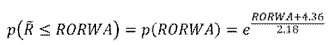
The inverse of this function, which
we will label p(RORWA), gives the probability that a particular
realization of RORWA,
Figure 4. DISPLAY EQUATION
$$
\tilde{R}
$$
will be less than or equal to a specified
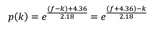
level over a given year. That function is:
Next, assume that a BHC becomes non-viable and consequently
defaults if and only if its capital ratio k (measured in terms
of common equity tier 1 capital, or CET1) falls to some failure point f. (Note that k is a variable and f is a constant.)
We assume that RORWA and k are independent, which is appropriate
because the return on an asset should not depend to a significant
extent on the identity of the entity holding the asset or on that
entity’s capital ratio. We can now estimate the probability that a
BHC with capital level k will suffer sufficiently severe losses
(that is, a negative RORWA of sufficiently great magnitude) to bring
its capital ratio down to the failure point f. We are looking
for the probability that k will fall to f, that is,
the probability that k + RORWA = f. Solving for RORWA,
we get RORWA = f - k, which we can then plug into the
function above to find the probability of default as a function of
the capital ratio k:11
We
can now create a function that takes as its input a GSIB’s LGD score
and produces a capital surcharge for that GSIB. In the course of doing
so, we will find that the resulting surcharges are invariant to both
the failure point f and the generally applicable capital level that
the GSIB surcharge is held on top of, which means that we do not need
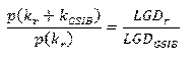
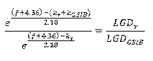
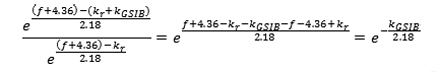
to make any assumption about the value of these two quantities. Recall
that the goal of the expected impact framework is to make the following
equation true:
ELGSIB = ELr
Let kr be the generally applicable
capital level held by the reference BHC, and let kGSIB be the GSIB surcharge that a given GSIB is required
to hold on top of kr. Thus, the reference
BHC’s probability of default will be p(kr) and each GSIB’s probability of default will be p(kr + kGSIB), with
the value of kGSIB varying from firm to
firm. Because EL = LGD * PD, the equation above
can be expressed as:
As promised, the failure point f and
the baseline capital level kr prove to be
irrelevant. This is a consequence of the assumption that the quantiles
of the RORWA distribution are linearly related to the logarithm of
the quantile. Thus, we have:
The appropriate surcharge for a given GSIB
depends only on that GSIB’s LGD score and the chosen reference BHC’s
LGD score. Indeed, the surcharge does not even depend on the particular
values of those two scores, but only on the ratio between them. Thus,
doubling, halving, or otherwise multiplying both scores by the same
constant will not affect the resulting surcharges. And since each
of our reference BHC options was determined in relation to the LGD
scores of actual firms, any multiplication applied to the calculation
of the firms’ LGD scores will also carry over to the resulting reference
BHC scores.
Note that the specific GSIB surcharge depends on the slope
coefficient that determines how the quantiles of the RORWA distribution
change as the probability changes. The empirical analysis presented
in figure 3 suggests a value for the slope coefficient of roughly
2.18; however, there is uncertainty regarding the true population
value of this coefficient. There are two important sources of uncertainty.
First, the estimated value of 2.18 is a statistical estimate that
is subject to sampling uncertainty. This sampling uncertainty is characterized
in terms of the standard error of the coefficient estimate, which
is 0.11 (as reflected in parentheses beneath the point estimate in
figure 3). Under standard assumptions, the estimated value of the
slope coefficient is approximately normally distributed with a mean of
2.18 and a standard deviation of 0.11. A 99 percent confidence interval
for the slope coefficient ranges from approximately 1.9 to 2.4.
Second, there is additional uncertainty around the slope
coefficient that arises from uncertainty as to whether the data sample
used to construct the estimated slope coefficient is indicative of
the RORWA distribution that will obtain in the future. As discussed
above, there are reasons to believe that the future RORWA distribution
will differ to some extent from the historical distribution. Accordingly,
the 99 percent confidence interval for the slope coefficient that
is presented above is a lower bound to the true degree of uncertainty
that should be attached to the slope coefficient.
We can now use the GSIB surcharge formula and
99 percent confidence interval presented above to compute the ranges
of capital surcharges that would obtain for each of the reference
BHC options discussed above. Table 2 presents method 1 surcharge ranges
and table 3 presents method 2 surcharge ranges. The low estimate in
each cell was computed using the surcharge formula above with the
value of the slope coefficient at the low end of the 99 percent confidence
interval (1.9); the high end was computed using the value of the slope
coefficient at the high end of that interval (2.4).
Table 2—Method
1 surcharge ranges for each reference BHC (%)
Firm
Method 1 score
$50 billion reference BHC
$250 billion reference BHC
Non-GSIB with highest LGD
Reference BHC LGD = 130
JPMorgan Chase
473
9.6,
12.4
5.7,
7.4
4.2,
5.5
2.5,
3.2
Citigroup
409
9.3,
12.1
5.5,
7.1
4.0,
5.1
2.2,
2.8
Bank of America
311
8.8,
11.4
4.9,
6.4
3.4,
4.4
1.7,
2.1
Goldman Sachs
248
8.4,
10.9
4.5,
5.8
3.0,
3.9
1.2,
1.6
Morgan Stanley
224
8.2,
10.6
4.3,
5.6
2.8,
3.6
1.0,
1.3
Wells Fargo
197
8.0,
10.3
4.1,
5.3
2.6,
3.3
0.8,
1.0
Bank of New York
Mellon
149
7.4,
9.6
3.6,
4.6
2.0,
2.6
0.3,
0.3
State Street
146
7.4,
9.6
3.5,
4.5
2.0,
2.6
0.2,
0.3
Reference score
3
23
51
130
Table 3—Method
2 surcharge ranges for each reference BHC (%)
Firm
Method 2 score
$50 billion reference BHC
$250 billion reference BHC
Non-GSIB with highest LGD
Reference BHC LGD = 100
JPMorgan Chase
857
6.0,
7.7
5.1,
6.5
4.4,
5.7
4.1,
5.3
Citgroup
714
5.6,
7.3
4.7,
6.1
4.0,
5.2
3.7,
4.8
Goldman Sachs
585
5.2,
6.8
4.3,
5.6
3.7,
4.7
3.4,
4.3
Bank of America
559
5.2,
6.7
4.2,
5.5
3.6,
4.6
3.3,
4.2
Morgan Stanley
545
5.1,
6.6
4.2,
5.4
3.5,
4.6
3.2,
4.2
Wells Fargo
352
4.3,
5.5
3.4,
4.4
2.7,
3.5
2.4,
3.1
State Street
275
3.8,
4.9
2.9,
3.7
2.2,
2.9
1.9,
2.5
Bank of New York
Mellon
213
3.3,
4.3
2.4,
3.1
1.7,
2.3
1.4,
1.9
Reference score
37
60
85
100
Surcharge Bands
The analysis above suggests a range of capital surcharges
for a given LGD score. To obtain a simple and easy-to-implement surcharge
rule, we will assign surcharges to discrete “bands” of scores so that
the surcharge for a given score falls in the lower end of the range
suggested by the results shown in tables 2 and 3. The bands will be
chosen so that the surcharges for each band rise in increments of
one half of a percentage point. This sizing will ensure that modest
changes in a firm’s systemic indicators will generally not cause a
change in its surcharge, while at the same time maintaining a reasonable
level of sensitivity to changes in a firm’s systemic footprint. Because
small changes in a firm’s score will generally not cause a change
to the firm’s surcharge, using surcharge bands will facilitate capital
planning by firms subject to the rule.
We will omit the surcharge band associated with a 0.5
percent surcharge. This tailoring for the least-systemic band of scores
above the reference BHC score is rational in light of the fixed costs
of imposing a firm-specific capital surcharge; these costs are likely
not worth incurring where only a small surcharge would be imposed.
(The internationally accepted GSIB surcharge framework similarly lacks
a 0.5 percent surcharge band.) Moreover, aminimum surcharge of 1.0
percent for all GSIBs accounts for the inability to know precisely
where the cut-off line between a GSIB and a non-GSIB will be at the
time when a failure occurs, and the surcharge’s purpose of enhancing
the resilience of all GSIBs.
We will use 100-point fixed-width bands, with a 1.0 percent
surcharge band at 130-229 points, a 1.5 percent surcharge band at 230-329 points, and so on. These surcharge bands fall in the lower
end of the range suggested by the results shown in tables 1 and 2.
The analysis above suggests that the surcharge should
depend on the logarithm of the LGD score. The logarithmic function
could justify bands that are smaller for lower LGD scores and larger
for higher LGD scores. For the following reasons, however, fixed-width
bands are more appropriate than expanding-width bands.
First, fixed-width surcharge bands
facilitate capital planning for less-systemic firms, which would otherwise
be subject to a larger number of narrower bands. Such small bands
could result in frequent and in some cases unforeseen changes in those
firms’ surcharges, which could unnecessarily complicate capital planning
and is contrary to the objective of ensuring that relatively small
changes in a firm’s score generally will not alter the firm’s surcharge.
Second, fixed-width surcharge bands are appropriate in
light of several concerns about the RORWA dataset and the relationship
between systemic indicators and systemic footprint that are particularly
relevant to the most systemically important financial institutions.
Larger surcharge bands for the most systemically important firms would
allow these firms to expand their systemic footprint materially within
the band without augmenting their capital buffers. That state of affairs
would be particularly troubling in light of limitations on the data
used in the statistical analysis above.
In particular, while the historical RORWA dataset used
to derive the function relating a firm’s LGD score to its surcharge
contains many observations for relatively small losses, it contains
far fewer observations of large losses of the magnitude necessary
to cause the failure of a firm that has a very large systemic footprint
and is therefore already subject to a surcharge of (for example) 4.0
percent. This paucity of observations means that our estimation of
the probability of such losses is substantially more uncertain than
is the case with smaller losses. This is reflected in the magnitude
of the standard error range associated with our regression analysis,
which is large and rapidly expanding for high LGD scores. Given this
uncertainty, as well as the Board’s Dodd-Frank Act mandate to impose
prudential standards that mitigate risks to financial stability, we
should impose a higher threshold of certainty on the sufficiency of
capital requirements for the most systemically important financial
institutions.
Two further shortcomings of the RORWA dataset make the
case for rejecting ever-expanding bands even stronger. First, the
frequency of extremely large losses would likely have been higher in
the absence of extraordinary government actions taken to protect financial
stability, especially during the 2007-08 financial crisis. As discussed
above, the GSIB surcharge should be set on the assumption that extraordinary
interventions will not recur in the future (in order to ensure that
they will not be necessary in the future), which means that firms
need to hold more capital to absorb losses in the tail of the distribution
than the historical data would suggest. Second, the historical data
are subject to survivorship bias, in that a given BHC is only included
in the sample until it fails (or is acquired). If a firm fails in
a given quarter, then its experience in that quarter is not included
in the dataset, and any losses realized during that quarter (including
losses realized only upon failure) are therefore left out of the dataset,
leading to an underestimate of the probability of such large losses.
Additionally, as discussed above, our assumption of a
linear relationship between a firm’s LGD score and the risk that its
failure would pose to financial stability likely understates the surcharge
that would be appropriate for the most systemically important firms.
As noted above, there is reason to believe that the damage to the
economy increases more rapidly as a firm grows in size, complexity,
reliance on short-term wholesale funding, and perhaps other GSIB metrics.
Finally, fixed-width bands are preferable to expanding-width
bands because they are simpler and therefore more transparent to regulated
entities and to the public.
Alternatives to the Expected Impact Framework
Federal Reserve staff considered various alternatives to the expected
impact framework for calibrating a GSIB surcharge. All available methodologies
are highly sensitive to a range of assumptions.
Economy-Wide Cost-Benefit Analysis
One
alternative to the expected impact framework is to assess all social
costs and benefits of capital surcharges for GSIBs and then set each
firm’s requirement at the point where marginal social costs equal
marginal social benefits. The principal social benefit of a GSIB surcharge
is a reduction in the likelihood and severity of financial crises
and crisis-induced recessions. Assuming that capital is a relatively
expensive source of funding, the potential costs of higher GSIB capital
requirements come from reduced credit intermediation by GSIBs (though
this would be offset to some extent by increased intermediation by
smaller banking organizations and other entities), a potential loss
of any GSIB scale efficiencies, and a potential shift of credit intermediation
to the less-regulated shadow banking sector. The GSIB surcharges that
would result from this analysis would be sensitive to assumptions
about each of these factors.
One study produced by the Basel Committee on Banking Supervision
(with contributions from Federal Reserve staff) finds that net social
benefits would be maximized if generally applicable common equity
requirements were set to 13 percent of risk-weighted assets, which
could imply that a GSIB surcharge of up to 6 percent would be socially
beneficial.12 The surcharges produced by the expected
impact framework are generally consistent with that range.
That said, cost-benefit analysis
was not chosen as the primary calibration framework for the GSIB surcharge
for two reasons. First, it is not directly related to the mandate
provided by the Dodd-Frank Act, which instructs the Board to mitigate
risks to the financial stability of the United States. Second, using
cost-benefit analysis to directly calibrate firm-specific surcharges
would require more precision in estimating the factors discussed above
in the context of surcharges for individual firms than is now attainable.
Offsetting the Too-Big-To-Fail
Subsidy
It is generally agreed that GSIBs enjoyed
a “too-big-to-fail” funding advantage prior to the crisis
and ensuing regulation, and some studies find that such a funding
advantage persists. Any such advantage derives from the belief of
some creditors that the government might act to prevent a GSIB from
defaulting on its debts. This belief leads creditors to assign a lower
credit risk to GSIBs than would be appropriate in the absence of this
government “subsidy,” with the result that GSIBs can borrow at lower
rates. This creates an incentive for GSIBs to take on even more leverage
and make themselves even more systemic (in order to increase the value
of the subsidy), and it gives GSIBs an unfair advantage over less
systemic competitors.
In theory, a GSIB surcharge could be calibrated to offset
the too-big-to-fail subsidy and thereby cancel out these undesirable
effects. The surcharge could do so in two ways. First, as with an
insurance policy, the value of a potential government intervention
is proportional to the probability that the intervention will actually
occur. A larger buffer of capital lowers a GSIB’s probability of default
and thereby makes potential government intervention less likely. Put
differently, a too-big-to-fail subsidy leads creditors to lower the
credit risk premium they charge to GSIBs; by lowering credit risk,
increased capital levels would lower the value of any discount in
the credit risk premium. Second, banking organizations view capital
as a relatively costly source of funding. If it is, then a firm with
elevated capital requirements also has a concomitantly higher cost
of funding than a firm with just the generally applicable capital
requirements. And this increased cost of funding could, if calibrated
correctly, offset any cost-of-funding advantage derived from the too-big-to-fail
subsidy.
A surcharge calibration intended to offset any too-big-to-fail
subsidy would be highly sensitive to assumptions about the size of
the subsidy and about the respective costs of equity and debt as funding
sources at various capital levels. These quantities cannot currently
be estimated with sufficient precision to arrive at capital surcharges
for individual firms. Thus, the expected impact approach is preferable
as a primary framework for setting GSIB surcharges.
Cf. Dodd-Frank Act section 165(a)(1), which instructs the Board to
apply more stringent prudential standards to certain large financial
firms “[i]n order to prevent or mitigate risks to the financial stability
of the United States that could arise from the material financial
distress or failure . . . of large, interconnected financial institutions.”
As illustrated by the financial crisis that led Congress to enact
the Dodd-Frank Act, financial instability can lead to a wide range
of social harms, including the declines in employment and GDP growth
that are associated with an economic recession.
These estimates were produced by plotting the estimated scores of
six U.S. BHCs with total assets between $50 billion and $100 billion
against their total assets, running a linear regression, and finding
the score implied by the regression for a $50 billion firm. These
firms’ scores were estimated using data from the sources described
in the general note to table 1, except that figures for the short-term
wholesale funding component of method 2 were estimated using FR Y-9C
data from the first quarter of 2015 and Federal Reserve quantitative
impact study (QIS) data as of the fourth quarter of 2014. Scores for
firms with total assets below $50 billion were not estimated (and
therefore were not included in the regression analysis) because the
Federal Reserve does not collect as much data from those firms.
These estimates were produced by applying the approach described
in footnote 5 to 10 U.S BHCs with total assets between $100 billion
and $400 billion. Bank of New York Mellon and State Street, which
have total assets within that range, were excluded from the sample
because they are GSIBs and the expected impact framework assumes that
the reference BHC is a non-GSIB.
These estimates were produced using data from the sources described
in the general note to table 1, except that figures for the short-term
wholesale funding component of method 2 were estimated using FR Y-9C
data from the first quarter of 2015 and Federal Reserve quantitative
impact study (QIS) data as of the fourth quarter of 2014.
Because Basel I risk-weighted assets data are only available from
1996 onward, risk-weighted assets data for earlier years are estimated
by back-fitting the post-1996 ratio between risk-weighted assets and
total assets onto pre-1996 total assets data. See Andrew Kuritzkes
and Til Schuermann (2008), “What We Know, Don’t Know, and Can’t Know
about Bank Risk: A View from the Trenches,” University of Pennsylvania,
Financial Institutions Center paper #06-05, http://fic.wharton.upenn.edu/fic/papers/06/0605.pdf.
The concept of risk aversion provides additional support for this
assumption. While the failure of a GSIB in any given year is unlikely,
the costs from such a failure to financial stability could be severe.
By contrast, any costs from higher capital surcharges will be distributed
more evenly among different states of the world. Presumably society
is risk-averse and, in a close case, would prefer the latter set of
costs to the former. While this paper does not attempt to incorporate
risk aversion into its quantitative analysis, that concept does provide
additional support for the decision not to discount the historical
probability of large losses in light of post-crisis regulatory reforms.
This paper treats dollars of risk-weighted assets as equivalent regardless
of whether they are measured under the risk weightings of Basel I
or of Basel III. This treatment makes sense because the two systems
produce roughly comparable results and there does not appear to be
any objectively correct conversion factor for converting between them.
See Basel Committee on Banking Supervision (2010), An Assessment
of the Long-Term Economic Impact of Stronger Capital and Liquidity
Requirements (Basel, Switzerland: Bank for International Settlements,
August), p. 29, www.bis.org/publ/bcbs173.pdf. The study finds that
a capital ratio of 13 percent maximizes net benefits on the assumption
that a financial crisis can be expected to have moderate permanent
effects on the economy.